Substitution

23.1 INTRODUCTION
- 23.1.1 Unveiling the First Fundamental Form
- 23.1.2 Distortion Factor and Integration, Again
23.2 LECTURE
23.3 EXAMPLES
EXERCISES

23.1 INTRODUCTION

23.1.1 Unveiling the First Fundamental Form

We have introduced a general notion of derivative of a function from . The determinant . was called the distortion factor. In the case of a map from of the same dimension, the distortion factor is simply because the now square matrix has the same determinant than and the determinant is multiplicative. The first fundamental form is also called the metric tensor. In general relativity it plays an important role. Before we start, let us say that instead of using as a coordinate change, we will use , the reason being that will be used in polar coordinates.

**Figure 1.** Coordinate changes even make it to main stream news. Here is a NBCnews page from 2011 reporting about "space-time warp. **Gravity probe B** (active between 2004 and 2010) carried two gyroscopes pointing to a star. The gyroscopes experienced small spin rotation changes matching the predictions of general relativity.

23.1.2 Distortion Factor and Integration, Again

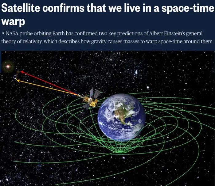
It describes a space in which distances are warped: it is matter in space that produces a coordinate change which changes the metric. How this happens is described by a complicated partial differential equation, the Einstein equations. We look here again at the distortion factor. The reason is that when we do integration in other coordinates, the distortion factor comes in. We will learn here how to integrate in polar coordinates or integrate in spherical coordinates.

23.2 LECTURE

23.2.1 Change of Variables Theorem

If is a coordinate change, then the distortion factor was defined as , where The change of variable theorem is the same in all dimensions. In the following proof, we assume that is . Because of Heine-Cantor, we know there exists with for and all .¹

Theorem 1. .

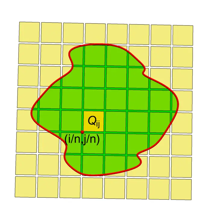
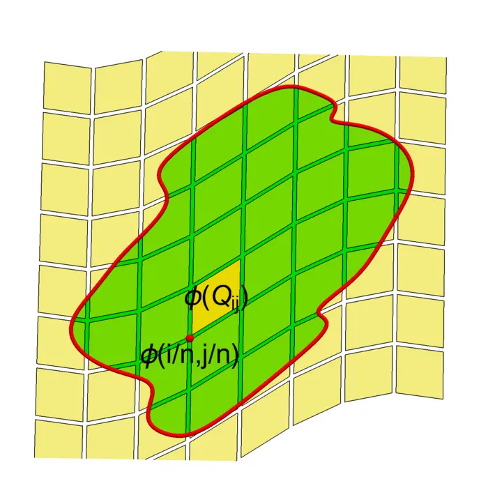
Proof. Cover with cubes as in the last lecture. Then The transformed squares are close to the parallelograms which have area . Now make a quadratic Taylor expansion at , where Let . Applying in every direction, Taylor with remainder, we see As the number of squares hitting is bound by where is the area of and is the length of the boundary of , the sum of the non-linear errors is therefore bound by which goes to zero for . ◻

23.2.2 Integrating a Disk with Change of Variables

Here is an example: If is given by , Then . If , then The first integral is .

23.2.3 Reversing Orientation

Let be given as . Now and . While we usually could ignore talking about orientation, it is evident here that the integrals considered so far, we do not care about the orientation of the space. If the change of coordinates switches the orientation, the resulting integral does not change.

23.2.4 Coordinate Changes and Elliptical Area Integrals

The chain rule assures that combining two coordinate changes , , gives a new coordinate change with For example if and changes into polar coordinates, then . Now the image of is the ellipse and the area of the ellipse is because and . The result is

23.2.5 Unveiling Surface Area with Parametrization

Preview: We will next week look at more general cases like of a parametrized surface, where the distortion factor is and the surface area is .

23.2.6 Change of Variables and Substitution

The theorem generalizes substitution if and . We usually insist that is monotonically increasing and write , to get computations like in where . As a hack, one can extend the formula to the case when can decrease in which case the interval becomes the negative interval with .
Example: Let which has , then In single variable calculus, one can also work with the negative sign case and compute which works if but this is not compatible with the defined Riemann integral: we use "spread-sheet" summation and do not distinguish whether we add up the function values from left to right or from right to left.

23.2.7 Fubini and Changing the Order of Integration

We can again look at the Fubini counter example We can not change the order of integration as we can not integrate . The trouble also continues in the new coordinate system and it is even more dramatic.

23.2.8 From Chain Rule to Matrix Products

If and are two linear coordinate changes then is the matrix product and the chain rule tells which agrees with the product . We can do the verification of the Cauchy-Binet formula directly. If then and you can check the determinant formula.

23.2.9 Open Problem: Inverses of Polynomial Coordinate Changes

Here is a famous open problem about coordinate changes. It is called the Jacobian conjecture. It deals with polynomial coordinate changes, where and are polynomials in , .

Conjecture: If is polynomial and is constant different from zero, then has a polynomial inverse.

One knows that if the conjecture is false, then there exists a counter example with integer polynomials and Jacobian determinant . The conjecture is open since at least 1939. An example of a coordinate transformation with determinant and integer polynomials are Hénon maps from lecture 16. If then

23.3 EXAMPLES

Example 1. Problem: What is the area of the image if and ? (This is with in the complex).
Solution: We have and . We see from the change of variables formula that the area is

Example 2. Problem: What is the moment of inertia , where is the polar region given in polar coordinates as .
Solution: using the polar coordinate change of variables with , we get We explain in class how to get the answer quickly.

Example 3. Problem: Here is a famous problem. It is so popular, that it even made it to Hollywood: compute .
Solution: this problem looks difficult at first as we can not integrate with respect to or . The function has no elementary anti-derivative. This improper integral is doable in polar coordinates as it is It is the inner part which is an improper integral. One deals with this by approximation. For every finite we have This converges nicely to for . It follows (and that is the punch line) that .

EXERCISES

Exercise 1. Given a disk , we can make this into a probability space and define the expectation of a function as The expectation of the random variables are examples of moments. Find , , and .

Exercise 2. What is the volume of the solid bound by and ? You can write this as a double integral over a suitable region.

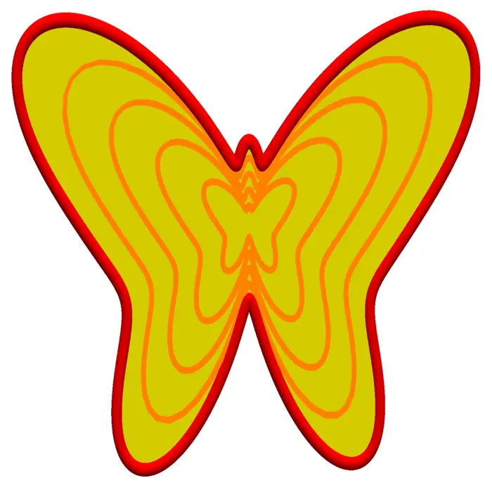
Exercise 3. The fidget spinner is so "" now. What is hot now is the math spinner with bearings! What is the moment of inertia of the math fidget spinner region given in polar coordinates as . To keep our bearings, we do not count the bearings.

Exercise 4. Biologist Piet Gielis once patented polar regions in order to use them to describe biological shapes like cells, leaves, starfish or butterflies. Don’t worry about violating patent laws when finding the area of the following butterfly (It can produce butterflies in your stomach but there are some tricks to do that fast. Relax with the Math fidget spinner for example!)

**Figure 3.** The math spinner and the butterfly.

Exercise 5.

Prove the Jacobian conjecture for linear maps , where is a matrix.
Find a linear coordinate change for which the Jacobian determinant is . It should be non-trivial in the sense, that we don’t just want a diagonal matrix .
Find a counter example of the Jacobian conjecture for cubic polynomials (just kidding). Find an example for the Jacobian conjecture where both polynomials are not linear!

For the case, see J. Schwartz, Mathematical Monthly 61, 1954, or P.D. Lax, Monthly 108, 2001.↩︎

Table of Contents