Extrema

19.1 INTRODUCTION
19.2 LECTURE
19.3 EXAMPLES
EXERCISES

19.1 INTRODUCTION

19.1.1 Exploring Learning as an Optimization Process

Learning is an optimization process with the goal to increase knowledge, skills and creative power. This applies both for education as well as for machine learning. In order to track the learning process, we need a function which measures progress. An old fashioned metric is the GPA averaging some grades in an educational system, an other or IQ scores measured by doing tests. An other metric example in a research setting is a social network score like the number of citations or the h-index. For a car driving autonomously it could be the where is the number of accidents produced using the parameter configuration in a fixed period.

**Figure 1.** The Klondike picture of David Perkins illustrates the search for solutions in a higher dimensional landscape defined by a height function . Calculus suggests to follow the gradient as this leads to **local maxima**. To find global maxima (which could be breakthrough ideas), we have to search harder and make a list of all maxima. The process is named after Klondike region in Canada which became infamous during the Gold rush.

19.1.2 Will AI Conquer Every Domain?

Once the frame work and the function is fixed, the question is how to increase most effectively. This simplistic picture is quite effective both for human intelligence or artificial intelligence. For many functions which have been considered (winning in chess games, computational power, data retention, feature detection, driving cars or flying planes) machines progressed rapidly. There is hardly anybody who seriously doubts that humans eventually will lose the battle for any function which can be considered. There are still domains where machines have not taken over. Examples are art or writing scientific papers.¹

19.1.3 Machine Learning’s Advantage in Gradient-Based Optimization

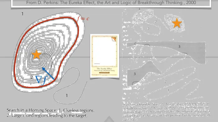
Once a machine knows the function , it can quit comfortably determine from a position in which direction to change to increase most rapidly. The direction of fastest increase is the direction of the gradient of . In calculus, we look at situations, where the position consists of a few variables only. Single variable calculus deals with the situation of one variable. We look here at the situation with variables but will mostly work with variables as this already gives the main idea. The principle is that we have reached an optimum where no change any more can increase the function . This means mathematically that the derivative of is zero. We call such points "critical points".

19.1.4 Using Gradients to Find the Direction of Improvement

Let us first look at the rate of change of a function along a direction . Take a curve where is a unit vector. By the chain rule, the rate of change at is given by We know for the dot product that this is equal to This is maximized for which means that points into the same direction than . So, The gradient points into the direction of maximal increase. This is important to remember. If you are in a landscape given by the height you have to go into the direction of in order to increase most. Of course, this does not make sense if but that is the situation where you are at a maximum, and where you can not increase any more.

19.2 LECTURE

19.2.1 Finding Optima with Gradients

All functions are assumed here to be in , meaning that they are two times continuously differentiable. It all starts with an observation going back to Pierre de Fermat:

Theorem 1. If is a maximum of , then .

Proof. We prove this by contradiction. Assume , define the vector and look at , which is a function of one variable. By the chain rule, it satisfies This means that for small . The point can not have been maximal. This is a contradiction. ◻

19.2.2 Unveiling Critical Points

A point with is called a critical point of . By the Taylor formula, we have at a critical point the quadratic approximation where is the Hessian matrix

19.2.3 The Second Derivative Test Steps In

As in one dimension, having a critical point does not assure that a point is a local maximum or minimum. The second derivative test in single variable calculus assures that if , , we have a local minimum and if , , we have a local maximum. If , we can not say anything without looking at higher derivatives.

19.2.4 Positive and Negative Definite Matrices

A matrix is called positive definite if for all vectors . It is called negative definite if for all vectors . A diagonal matrix with positive diagonal entries is positive definite. In the following statements, we assume is a critical point.

19.2.5 Unveiling the Role of Positive Definite Hessians

We say is a local maximum of if there exists such that for all . We say, it is a local minimum of if for all . How can we check whether a point is a local maximum or minimum?

Theorem 2. Assume . If is positive definite, then is a local minimum. If is negative definite, then is a local maximum.

Proof. As , the quadratic approximation at is for small non-zero and Hessian . The analogue statement for the minimum can be deduced by replacing with . ◻

19.2.6 Classifying Extrema in Two Dimensions

Let us look at the case, where is a function of two variables such that and . The Hessian matrix is

In this two dimensional case, we can classify the critical points if the determinant of is non-zero. The number is also called the discriminant at a critical point.

**Figure 2.** gives a minimum, a maximum and a saddle. The case is not Morse.

19.2.7 Morse Functions and the Second Derivative Test

We say is a Morse point, if is a critical point and the determinant is non-zero. A function is a Morse function if every critical point is Morse. Examples of Morse functions are , and . The last case is called a hyperbolic saddle. In general, a critical point is a hyperbolic saddle if and if it is neither a maximum nor a minimum. Here is the second derivative test in dimension :

Theorem 3. Assume has a critical point with .

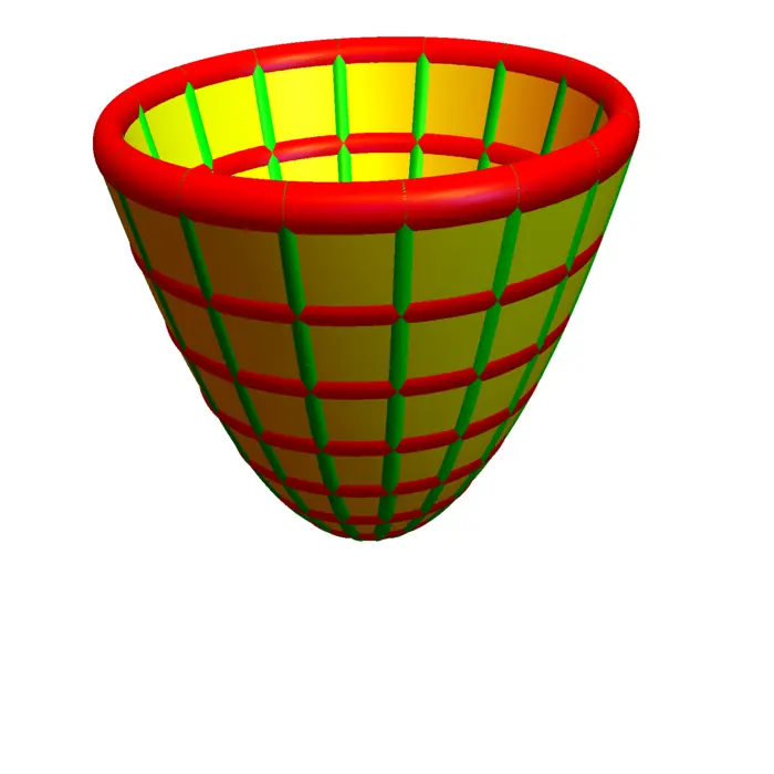
If and then is a local minimum.
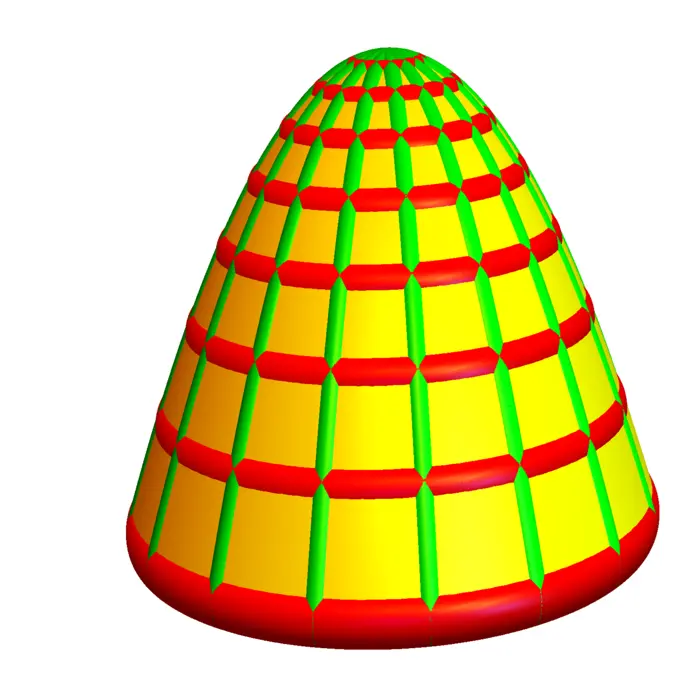
If and then is a local maximum.
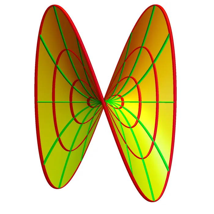
If then is a hyperbolic saddle.

Proof. After translation and replacing with , we have and . At the critical point, the quadratic approximation is now This can be rewritten as with and discriminant . If and then and the function has positive values for all . The point is then a minimum. If and , then and the function has negative values for all and the point is a local maximum. If , then takes both negative and positive values near . ◻

19.2.8 From Hessian to Gauss Curvature

One can ask, why and not is chosen. It does not matter, because if , then both and need to be non-zero and have the same sign. Instead of , one could also have pick the more natural trace . It is invariant under coordinate changes similarly as the determinant . The discriminant happens also to be the Gauss curvature of the surface at the point.

19.2.9 The Morse Lemma

In higher dimensions, the situation is described by the Morse lemma. It tells that near a critical point there is a coordinate change such that is a quadratic function where is diagonal with entries or . Critical point can then be given a Morse index, the number of entries in . The Morse lemma is actually a theorem (theorems are more important than lemmata=helper theorems)

Theorem 4. Near a Morse critical point of a function , there is a coordinate change such that is

Proof. We use induction with respect to .

Induction foundation: For , the result tells that for a Morse critical point, the function looks like or . First show that if , , then or for some positive function . Proof. By a linear coordinate change we assume and . There exists then such that : it is for and is in the limit the value of . By the product rule, with . Because can define for and take the limit , because by applying Hôpital twice, the limit is . The coordinate change is now given by a function satisfying . Implicit differentiation gives so that by the implicit function theorem exists.
Induction step : we first note that Taylor for with remainder term implies that with some continuous functions . Furthermore, the function value are the coordinates of the Hessian. Apply first a rotation so that . Now look at and keep the other coordinates constant. As in (i), find a coordinate change such that , where inherits the properties of but is of one dimension less. By induction assumption, there is a second coordinate change such that Combining and produces the Morse normal form.

◻

19.3 EXAMPLES

Example 1. Q: Classify the critical points of .
A: As the critical points are , , and . We compute For and we have and so saddle points. For , we have , , a local max. For where , we have a local min.

EXERCISES

Exercise 1.

Classify the critical points of the function (Maxima, minima or saddle points).
Now do the same for and find the Morse index at each critical point.

Exercise 2. Find all critical points of the D area function Compute the Hessian at each critical point and determine the maxima (all eigenvalues are negative) and minima (all eigenvalues are positive).
P.S. Area is an old hat. But D Area is still highly classified and rumored to be near the dark side of the moon.

Exercise 3. Where on the parametrized surface is the temperature minimal. Classify all the critical points of the function . [If you have found the function , you can replace , again with , if you like to work with a function .]

Exercise 4. Find all the critical points of the function In each of the cases, find the Hessian matrix. Also here compute the eigenvalues. These are numbers such that for some non-zero vector. One can find them by looking for the roots of the characteristic polynomial . You can calculate them on a computer. Find in each case the eigenvalues.

Exercise 5.

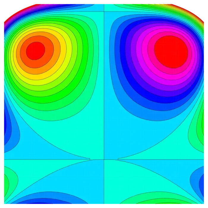
Find a function with maxima and saddle points and one minimum.
You see below a contour map of a function of two variables. How many critical points are there? Is the function a Morse function?

There could be resistance: humans might decide not to cite scientific breakthroughs by machines. On the other hand, who would not want to learn a "theory of everything" even if it is discovered by a machine?↩︎

Table of Contents