Constraints

20.1 INTRODUCTION
- 20.1.1 Gradients for Optimal Solutions with Constraints
- 20.1.2 Lagrange’s Magic: Many Constraints, One Solution
20.2 LECTURE
20.3 EXAMPLES
EXERCISES
Appendix: Data illustration: Cobb Douglas
- 20.3.1 Cobb-Douglas: A Formula for Economic Growth
- 20.3.2 Visualizing Production Limits

20.1 INTRODUCTION

20.1.1 Gradients for Optimal Solutions with Constraints

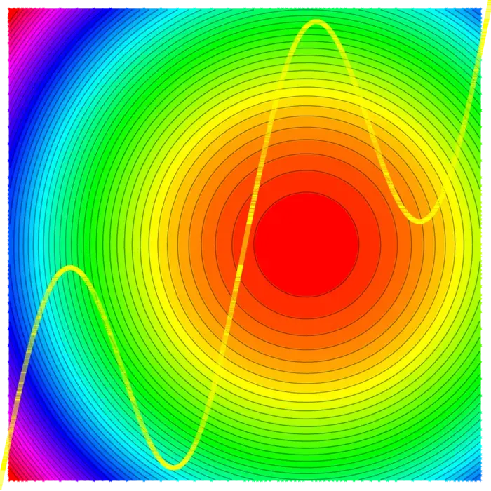
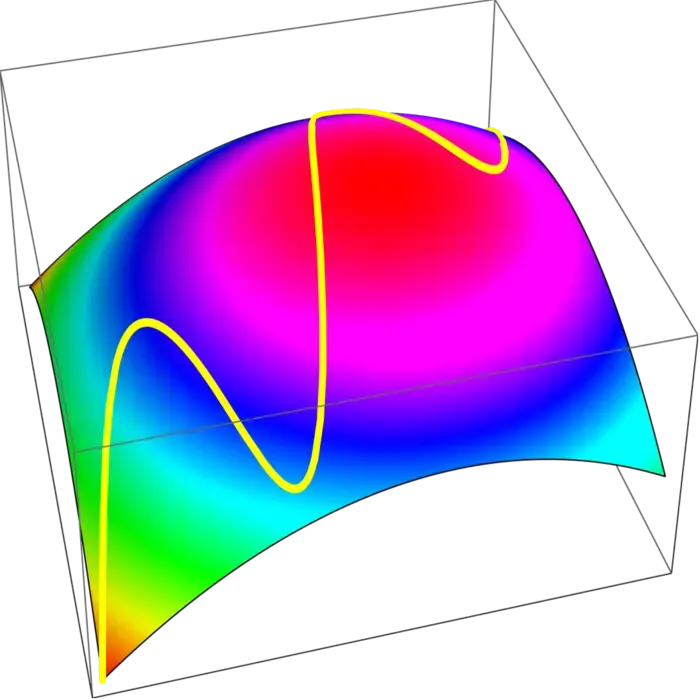
There is rarely a "free lunch". If we want to maximize a quantity, we often have to work with constraints. Obstacles might prevent us to change the parameters arbitrarily. The gradient can still be used as a guiding principle. While we can not achieve to be zero, we can look for points where the gradient is perpendicular to the constraint. This gives us an optimal point under the confinement. If you hike on a path in the mountains, you often reach a local maximum without being on top of the mountain. What happens at such points is that is perpendicular to the curve meaning that is parallel to .

**Figure 1.** The situation, where a function is optimized along a curve is a frame-work which can be tackled with Lagrange. The condition of being maximal means that the gradient of is perpendicular to the curve. This means that the gradients of and are parallel. .

20.1.2 Lagrange’s Magic: Many Constraints, One Solution

The method of Lagrange is much more general. We can work with arbitrary many constraints and still use the same principle. The gradient of is then perpendicular to the constraint surface which means that is a linear combination of the gradients of all the constraints: these are equations because the vectors have components. Together with the equations we have equations for variables , .

20.2 LECTURE

20.2.1 Finding the Maximum in Confined Spaces

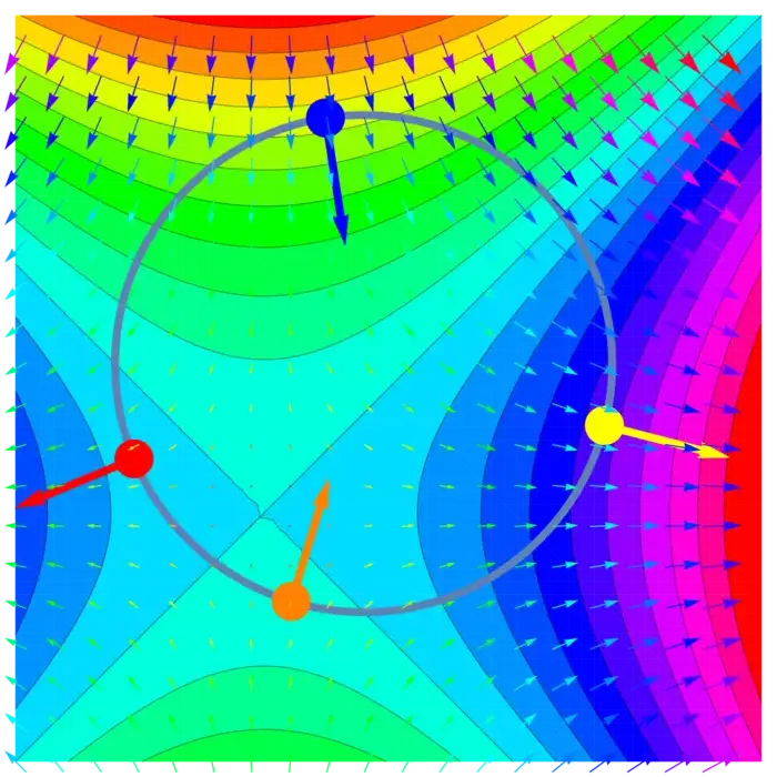
If we want to maximize a function on the constraint then both the gradients of and matter. We call two vectors , parallel if or for some real . The zero vector is parallel to everything. Here is a variant of Fermat:

Theorem 1. If is a maximum of under the constraint , then and are parallel.

Proof. By contradiction: assume and are not parallel and is a local maximum. Let be the tangent plane to at . Because is not perpendicular to we can project it onto to get a non-zero vector in which is not perpendicular to . Actually the angle between and is acute so that . Take a curve in with and . We have By linear approximation, we know that for small enough . This is a contradiction to the fact that was maximal at on . ◻

20.2.2 Exploring Lagrange Multipliers and Necessary Conditions

This immediately implies: (distinguish and )

Theorem 2. For a maximum of on either the Lagrange equations , hold, or then , .

For functions of two variables, this means we have to solve a system with three equations and three unknowns:

20.2.3 Finding the True Maximum

To find a maximum, solve the Lagrange equations and add a list of critical points of on the constraint. Then pick a point where is maximal among all points. We don’t bother with a second derivative test. But here is a possible statement: for all perpendicular to , then is a local maximum.

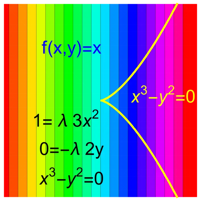
Of course, the case of maxima and minima are analog. If has a maximum on , then has a minimum at . We can have a maximum of under a smooth constraint without that the Lagrange equations are satisfied. An example is and shown in Figure (20.3).

**Figure 3.** An example of a function, where the Lagrange equations do not give the minimum, here . It is a case, where .

20.2.4 Lagrange’s Climb: Maximizing with Multiple Constraints

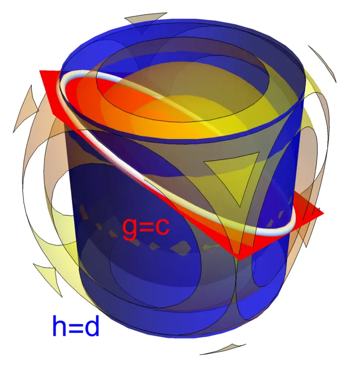
The method of Lagrange can maximize functions under several constraints. Lets show this in the case of a function of three variables and two constraints and . The analogue of the Fermat principle is that at a maximum of , the gradient of is in the plane spanned by and . This leads to the Lagrange equations for unknowns .

For example, if then we find points on the ellipse , with minimal or maximal distance to .

**Figure 4.** We see a situation where we try to maximize a function under two constraints. In this case the intersection , is an ellipse.

20.3 EXAMPLES

Example 1. Problem: Minimize under the constraint .
Solution: The Lagrange equations are , . If then . If we can divide the second equation by and get , again showing . The point , is the only solution.

Example 2. Problem: Which cylindrical soda can of height and radius has minimal surface for fixed volume ?
Solution: We have and . With , , you need to optimize under the constrained . We will do that in class.

Example 3. Problem: If is the probability that a dice shows , then we have . This vector is called a probability distribution. The Shannon entropy of is defined as

Find the distribution which maximizes entropy .
Solution: The Lagrange equations are from which we get . The last equation fixes so that . It is the fair dice that has maximal entropy. Maximal entropy means least information content.

Example 4. Assume that the probability that a physical or chemical system is in a state is and that the energy of the state is . Nature minimizes the free energy if the energies are fixed. The probability distribution satisfying minimizing the free energy is called a Gibbs distribution. Find this distribution in general if are given.
Solution: The Lagrange equation are , or , where . The constraint gives so that . The Gibbs solution is .¹

Example 5. If is a quadratic function on and is linear that is with and if the constraint is linear , then and . Lets call . The Lagrange equations are then , . We see in general that for quadratic and linear , we end up with a linear system of equations.

Example 6. Related to the previous remark is the following observation. It is often possible to reduce the Lagrange problem to a problem without constraint. This is a point of view often taken in economics. Let us look at it in dimension , where we extremize under the constraint . Define . The Lagrange equations for are now equivalent to in three dimensions.

EXERCISES

Exercise 1. Find the cylindrical basket which is open on the top has has the largest volume for fixed area . If is the radius and is the height, we have to maximize under the constraint Use the method of Lagrange multipliers.

Exercise 2. Given a symmetric matrix , we look at the function . and look at extrema of under the constraint that . This leads to an equation A solution is called an eigenvector. The Lagrange constant is an eigenvalue. Find the solutions to , if is a matrix, where Then solve the problem with , , , .

Exercise 3. Which pyramid of height over a square with surface area is has maximal volume ? By using new variables and multiplying with a constant, we get to the equivalent problem to maximize over the constraint Use the later variables.

Exercise 4. Motivated by the Disney movie "Tangled", we want to build a hot air balloon with a cuboid mesh of dimension , , which together with the top and bottom fortifications uses wires of total length Find the balloon with maximal volume .

Exercise 5. A solid bullet made of a half sphere and a cylinder has the volume and surface area . Doctor Manhattan designs a bullet with fixed volume and minimal area. With and he therefore minimizes under the constraint Use the Lagrange method to find a local minimum of under the constraint .

Appendix: Data illustration: Cobb Douglas

20.3.1 Cobb-Douglas: A Formula for Economic Growth

The mathematician and economist Charles W. Cobb at Amherst college and the economist and politician Paul H. Douglas who was also teaching at Amherst, found in 1928 empirically a formula which fits the total production of an economic system as a function of the capital investment and the labor . The two authors used logarithms variables and assumed linearity to find . Below are the data normalized so that the date for year 1899 has the value .

Year
1899	100	100	100
1900	107	105	101
1901	114	110	112
1902	122	118	122
1903	131	123	124
1904	138	116	122
1905	149	125	143
1906	163	133	152
1907	176	138	151
1908	185	121	126
1909	198	140	155
1910	208	144	159
1911	216	145	153
1912	226	152	177
1913	236	154	184
1914	244	149	169
1915	266	154	189
1916	298	182	225
1917	335	196	227
1918	366	200	223
1919	387	193	218
1920	407	193	231
1921	417	147	179
1922	431	161	240

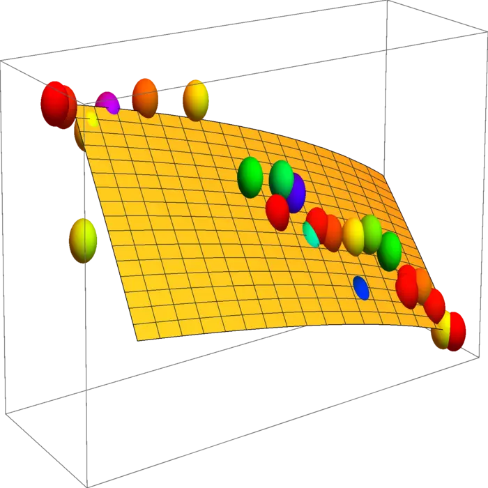
**Figure 5.** The graph of fits pretty well that data set. You can see in the data that there is an out-layer.

20.3.2 Visualizing Production Limits

Assume that the labor and capital investment are bound by the additional constraint . (This function is unrelated to the function as we are in a Lagrange problem.) Where is the production maximal under this constraint? Plot the two functions and .

This example is from Rufus Bowen, Lecture Notes in Math, 470, 1978↩︎

Table of Contents