Partial Differential Equations

13.1 INTRODUCTION
- 13.1.1 Math of Motion
13.2 LECTURE
13.3 ILLUSTRATION
EXERCISES

13.1 INTRODUCTION

13.1.1 Math of Motion

If we can relate the changes in one quantity with changes in an other quantity, partial differential equations come in. One of the simplest rules is that the rate of change of a function $f (t, x)$ in time is related to the rate of change in space. Such a rule could be expressed for example as a rule $f_{t} (t, x) = f_{x} (t, x)$ , where $f_{t}$ is the partial derivative with respect to $t$ and $f_{x}$ is the partial derivative with respect to $x$ . You can check that $f (t, x) = \sin (t + x)$ is an example of a function which satisfies this differential equation. You can see even that for any function $g$ , the function $f (t, x) = g (t + x)$ satisfies $f_{t} = f_{x}$ . A typical situation is to be given $f (0, x)$ , the situation of "now". We then can see what $f (t, x)$ is for a later time $t$ . This describes the situation in the future. As you see, the differential equation $f_{t} = f_{x}$ describes "transport". The initial situation is translated to the left. Check this out and draw for example $f (0, x) = x^{2}$ . We see that $f (t, x) = (x + t)^{2}$ and especially $f (1, x) = (x + 1)^{2}$ . The graph has moved to the left.

Illustration for Partial Differential Equations — **Figure 1.** A function $f (t, x)$ satisfying a differential equation $f_{t t} - f_{x x} = \sin (u)$ . This PDE is called *Sin-Gordon* equation, a nonlinear wave equation featuring **solitons**. Space is here one dimensional time goes from left to right. We see a wave going left and right, reflecting at the boundary and building up to a larger peak. A "rogue wave".

13.2 LECTURE

13.2.1 How PDEs Shape Our World

A partial differential equation is a rule which combines the rates of changes of different variables. Our lives are affected by partial differential equations: the Maxwell equations describe electric and magnetic fields $E$ and $B$ . Their motion leads to the propagation of light. The Einstein field equations relate the metric tensor $g$ with the mass tensor $T$ . The Schrödinger equation tells how quantum particles move. Laws like the Navier-Stokes equations govern the motion of fluids and gases and especially the currents in the ocean or the winds in the atmosphere. Partial differential equations appear also in unexpected places like in finance, where for example, the Black-Scholes equation relates the prices of options in dependence of time and stock prices.

13.2.2 Some Examples of PDEs and ODEs

If $f (x, y)$ is a function of two variables, we can differentiate $f$ with respect to both $x$ or $y$ . We just write $f_{x} (x, y)$ for $\partial_{x} f (x, y)$ . For example, for $f (x, y) = x^{3} y + y^{2}$ , we have $f_{x} (x, y) = 3 x^{2} y$ and $f_{y} (x, y) = x^{3} + 2 y$ . If we first differentiate with respect to $x$ and then with respect to $y$ , we write $f_{x y} (x, y)$ . If we differentiate twice with respect to $y$ , we write $f_{y y} (x, y)$ . An equation for an unknown function $f$ for which partial derivatives with respect to at least two different variables appear is called a partial differential equation PDE. If only the derivative with respect to one variable appears, one speaks of an ordinary differential equation ODE. An example of a PDE is $f_{x}^{2} + f_{y}^{2} = f_{x x} + f_{y y}$ , an example of an ODE is f^{\prime \prime}=f^{2}-f^{\prime}. It is important to realize that it is a function we are looking for, not a number. The ordinary differential equation f^{\prime}=3 f for example is solved by the functions $f (t) = C e^{3 t}$ . If we prescribe an initial value like $f (0) = 7$ , then there is a unique solution $f (t) = 7 e^{3 t}$ . The KdV partial differential equation $f_{t} + 6 f f_{x} + f_{x x x} = 0$ is solved by (you guessed it) $2 {sech}^{2} (x - 4 t)$ . This is one of many solutions. In that case they are called solitons, nonlinear waves. Korteweg-de Vries (KdV) is an icon in a mathematical field called integrable systems which leads to insight in ongoing research like about rogue waves in the ocean.

13.2.3 A Look at Clairaut’s Theorem for Mixed Derivatives

We say $f \in C^{1} (ℝ^{2})$ if both $f_{x}$ and $f_{y}$ are continuous functions of two variables and $f \in C^{2} (ℝ^{2})$ if all $f_{x x}$ , $f_{y y}$ , $f_{x y}$ and $f_{y x}$ are continuous functions. The next theorem is called the Clairaut theorem. It deals with the partial differential equation $f_{x y} = f_{y x}$ . The proof demonstrates the proof by contradiction. We will look at this technique a bit more in the proof seminar.

Theorem 1. Every $f \in C^{2}$ solves the Clairaut equation $f_{x y} = f_{y x}$ .

Proof. We use Fubini’s theorem which will appear later in the double integral lecture: integrate $\int_{x_{0}}^{x_{0} + h} (\int_{y_{0}}^{y_{0} + h} f_{x y} (x, y) d y) d x$ by applying the fundamental theorem of calculus twice \begin{aligned} &\int_{x_{0}}^{x_{0}+h} \big(f_{x}(x, y_{0}+h)-f_{x}(x, y_{0})\big) d x\\ =&f(x_{0}+h, y_{0}+h)-f(x_{0}, y_{0}+h)-f(x_{0}+h, y_{0})+f(x_{0}, y_{0}). \end{aligned} An analogous computation gives \begin{aligned} &\int_{y_{0}}^{y_{0}+h}\left(\int_{x_{0}}^{x_{0}+h} f_{y x}(x, y) \,d x\right) d y\\ =&f(x_{0}+h, y_{0}+h)-f(x_{0}, y_{0}+h)-f(x_{0}+h, y_{0})+f(x_{0}, y_{0}). \end{aligned} Fubini applied to $g (x, y) = f_{x y} (x, y)$ assures $\int_{y_{0}}^{y_{0} + h} (\int_{x_{0}}^{x_{0} + h} f_{y x} (x, y) d x) d y = \int_{x_{0}}^{x_{0} + h} (\int_{y_{0}}^{y_{0} + h} f_{y x} (x, y) d y) d x$ so that $\iint_{A} (f_{x y} - f_{y x}) d y d x = 0$ . $Assume$ there is some $(x_{0}, y_{0})$ , where $F (x_{0}, y_{0}) = f_{x y} (x_{0}, y_{0}) - f_{y x} (x_{0}, y_{0}) = c > 0,$ then also for small $h$ , the function $F$ is bigger than $c / 2$ everywhere on $A = [x_{0}, x_{0} + h] \times [y_{0}, y_{0} + h]$ so that $\iint_{A} F (x, y) d x d y \geq area (A) c / 2 = h^{2} c / 2 > 0$ $contradicting$ that the integral is zero. ◻

13.2.4 Why continuous differentiability Isn’t Enough for Clairaut’s Theorem

The statement is false for functions which are only $C^{1}$ . The standard counter example is $f (x, y) = 4 x y (y^{2} - x^{2}) / (x^{2} + y^{2})$ which has for $y \neq 0$ the property that $f_{x} (0, y) = 4 y$ and for $x \neq 0$ has the property that $f_{y} (x, 0) = - 4 x$ . You can see the comparison of $f (x, y) = 2 x y = r^{2} \sin (2 θ)$ and $f (x, y) = 4 x y (y^{2} - x^{2}) / (x^{2} + y^{2}) = r^{2} \sin (4 θ) .$ The later function is not in $C^{2}$ . The values $f_{x y}$ and $f_{y x}$ , changes of slopes of tangent lines, turn differently.

13.3 ILLUSTRATION

13.3.1 An Approach to Solving Transport Equations

In many cases, one of the variables is time for which we use the letter $t$ and keep $x$ as the space variable. The differential equation $f_{t} (t, x) = f_{x} (t, x)$ is called the transport equation. What are the solutions if $f (0, x) = g (x)$ ? Here is a cool derivation: if D f=f^{\prime} is the derivative,¹ we can build operators like (D+D^{2}+4 D^{4}) f=f^{\prime}+f^{\prime \prime}+4 f^{\prime \prime \prime \prime}. The transport equation is now $f_{t} = D f$ . Now as you know from calculus, the only solution of f^{\prime}=a f, $f (0) = b$ is $b e^{a t}$ . If we boldly replace the number $a$ with with the operator $D$ we get f^{\prime}=D f and get its solution \begin{aligned} e^{D t} g(x) &=\big(1+D t+D^{2} t^{2} / 2 !+\cdots\big) g(x)\\ &=g(x)+g^{\prime}(x) t+g^{\prime \prime}(x) t^{2} / 2 !+\cdots. \end{aligned} By the Taylor formula, this is equal to $g (x + t)$ . You should actually remember Taylor as $g (x + t) = e^{D t} g (x)$ . We have derived for $g (x) = f (0, x)$ in $C^{1} (ℝ^{2})$ :

Theorem 2. $f_{t} = f_{x}$ is solved by $f (t, x) = g (x + t)$ .

Proof. We can ignore the derivation and verify this very quickly: the function satisfies $f (0, x) = g (x)$ and $f_{t} (t, x) = f_{x} (t, x)$ . ◻

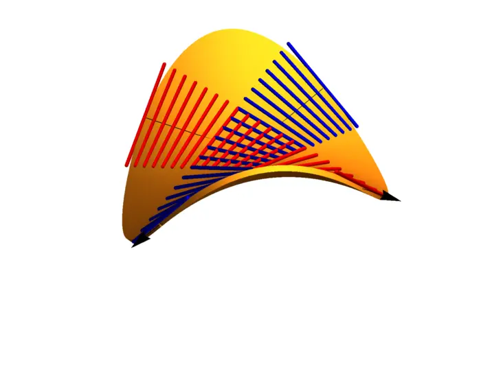
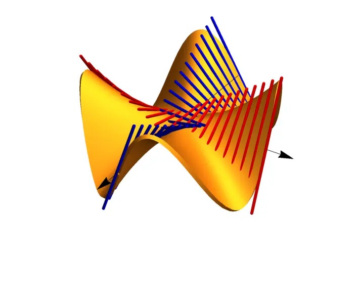
13.3.2 Solving the Wave Equation with D’Alembert’s Formula

Another example of a partial differential equation is the wave equation $f_{t t} =$ $f_{x x}$ . We can write this $(\partial_{t} + D) (\partial_{t} - D) f = 0$ . One way to solve this is by looking at $(\partial_{t} - D) f = 0$ . This means transport $f_{t} = f_{x}$ and $f (t, x) = f (x + t)$ . We can also have $(\partial_{t} + D) f = 0$ which means $f_{t} = - f_{x}$ leading to $f (x - t)$ . We see that every combination $a f (x + t) + b f (x - t)$ with constants $a, b$ is a solution. Fixing the constants $a, b$ so that $f (x, 0) = g (x)$ and $f_{t} (x, 0) = h (x)$ gives the following d’Alembert solution. It requires $g, h \in C^{2} (ℝ)$ .

Theorem 3. $f_{t t} = f_{x x}$ is solved by $f (t, x) = \frac{g (x + t) + g (x - t)}{2} + \frac{h (x + t) - h (x - t)}{2}$ .

Proof. Just verify directly that this indeed is a solution and that $f (0, x) = g (x)$ and $f_{t} (0, x) = h (x)$ . Intuitively, if we throw a stone into a narrow water way, then the waves move to both sides. ◻

13.3.3 From Heat Flow to Normal Distribution

The partial differential equation $f_{t} = f_{x x}$ is called the heat equation. Its solution involves the normal distribution $N (m, s) (x) = e^{- (x - m)^{2} / (2 s^{2})} / \sqrt{2 π s^{2}}$ in probability theory. The number $m$ is the average and $s$ is the standard deviation.

13.3.4 Solving the Heat Equation

If the initial heat $g (x) = f (0, x)$ at time $t = 0$ is continuous and zero outside a bounded interval $[a, b]$ , then

Theorem 4. $f_{t} = f_{x x}$ is solved by $f (t, x) = \int_{a}^{b} g (m) N (m, \sqrt{2 t}) (x) d m$ .

Proof. For every fixed $m$ , the function $N (m, \sqrt{2 t}) (x)$ solves the heat equation.

$\texttt{\footnotesize{{f}={PDF}[ NormalDistribution [{m}, \textbf{Sqrt}[2 {t}]], {x}]; {\textbf{Simplify}}[{\textbf{D}}[{f}, {t}]=={\textbf{D}}[{f},{{x}, 2}]] }}$

Every Riemann sum approximation $g (x) = (1 / n) \sum_{k = 1}^{n} g (m_{k})$ of $g$ defines a function $f_{n} (t, x) = (1 / n) \sum_{k = 1}^{n} g (m_{k}) N (m_{k}, \sqrt{2 t}) (x)$ which solves the heat equation. So does $f (t, x) = lim_{n \to \infty} f_{n} (t, x) .$ To check $f (0, x) = g (x)$ which need $\int_{- \infty}^{\infty} N (m, s) (x) d x = 1$ and $\int_{- \infty}^{\infty} h (x) N (m, s) (x) d x \to h (m)$ for any continuous $h$ and $s \to 0$ , proven later. ◻

13.3.5 The Role of Laplace’s Equation

For functions of three variables $f (x, y, z)$ one can look at the partial differential equation $Δ f (x, y, z) = f_{x x} + f_{y y} + f_{z z} = 0$ . It is called the Laplace equation and $Δ$ is called the Laplace operator. The operator appears also in one of the most important partial differential equations, the Schrödinger equation $i ℏ f_{t} = H f = - \frac{ℏ^{2}}{2 m} Δ f + V (x) f,$ where $ℏ = h / (2 π)$ is a scaled Planck constant and $V (x)$ is the potential depending on the position $x$ and $m$ is the mass. For $i ℏ f_{t} = P f$ with $P = - i ℏ D$ , then the solution $f (x - t)$ is forward translation. The operator $P$ is the momentum operator in quantum mechanics. The Taylor formula tells that $P$ generates translation.

EXERCISES

Exercise 1. Verify that for any constant $b$ , the function $f (x, t) = e^{- b t} \sin (x + t)$ satisfies the driven transport equation $f_{t} (x, t) = f_{x} (x, t) - b f (x, t) .$ This PDE is sometimes called the advection equation with damping $b$ .

Exercise 2. We have seen in class that $f (t, x) = e^{- x^{2} / (4 t)} / \sqrt{4 π t}$ solves the heat equation $f_{t} = f_{x x}$ . Verify more generally that $e^{- x^{2} / (4 a t)} / \sqrt{4 a π t}$ solves the heat equation $f_{t} = a f_{x x} .$

Exercise 3. The Eiconal equation $f_{x}^{2} + f_{y}^{2} = 1$ is used in optics. Let $f (x, y)$ be the distance to the circle $x^{2} + y^{2} = 1$ . Show that it satisfies the eiconal equation.

Remark: the equation can be written rewritten as $‖ d f ‖^{2} = 1$ , where $d f = \nabla f = [f_{x}, f_{y}]$ is the gradient of $f$ which is the Jacobian matrix for the map $f : ℝ^{2} \to ℝ$ .

Exercise 4. The differential equation $f_{t} = f - x f_{x} - x^{2} f_{x x}$ is a version of the Black-Scholes equation. Here $f (x, t)$ is the price of a call option and $x$ is the stock price and $t$ is time. Find a function $f (x, t)$ solving it which depends both on $x$ and $t$ .

Hint: look first for solutions $f (x, t) = g (t)$ or $f (x, t) = h (x)$ and then for functions of the form $f (x, t) = g (t) + h (x)$ .

Exercise 5. The partial differential equation $f_{t} + f f_{x} = f_{x x}$ is called Burgers equation and describes waves at the beach. In higher dimensions, it leads to the Navier-Stokes equation which is used to describe the weather. Verify that the function $f (t, x) = \frac{(\frac{1}{t})^{3 / 2} x e^{- \frac{x^{2}}{4 t}}}{\sqrt{\frac{1}{t}} e^{- \frac{x^{2}}{4 t}} + 1}$ is a solution of the Burgers equation. You better use technology.

We usually write $d f$ for derivative but $D$ tells it is an operator. D also stands for Dirac.↩︎

Table of Contents