Coordinates

10.1 INTRODUCTION
- 10.1.1 Algebraic Foundations of Coordinate Systems
10.2 LECTURE
10.3 EXAMPLES
10.4 ILLUSTRATIONS
- 10.4.1 Mandelbrot’s Complexity
- 10.4.2 Mandelbrot to Mandelbulb
EXERCISES

10.1 INTRODUCTION

10.1.1 Algebraic Foundations of Coordinate Systems

Algebra is a powerful tool in geometry. In this lecture we circle back to the concept of coordinates and look also at other coordinate systems. We have introduced space as column vectors like . We can think of it as an arrow from the origin to the point . One speaks of the numbers appearing in as coordinates while the entries in are components of the vector. Most of the time we do not distinguish between the point and the vector as the two objects can clearly be identified naturally. We look in this lecture also at other coordinates like Polar and spherical coordinates. This will be important when doing integration.

**Figure 1.** Napoleon’s theorem tells that if we draw equilateral triangles over the sides of a triangle, their center of mass are on an equilateral triangle. A geometric proof is not so easy to find but using coordinates it is a direct calculation: for three complex numbers , then , , satisfy . The result is famous because no other theorem has been rediscovered so many times. While Napoleon might never have discovered or proved it himself, he kept conversations with mathematicians like Lagrange or Fourier.

**Figure 2.** In the two-dimensional plane a point can also be identified with the complex number or the vector . The magnitude of the vector is and is defined to be the length of the complex number . Multiplication rotates and scales. A multiplication with rotates by degrees.

10.2 LECTURE

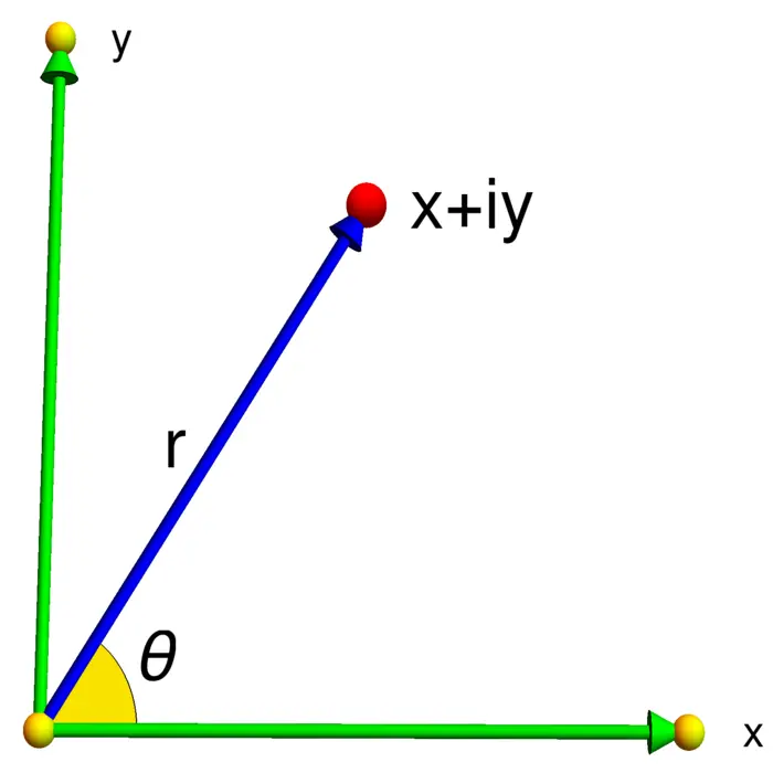
10.2.1 From Cartesian to Polar: A Coordinate Transformation

It was René Descartes who in 1637 introduced coordinates and brought algebra close to geometry.¹ The Cartesian coordinates in can be replaced by other coordinate systems like polar coordinates , where is the radial distance to the and is the polar angle made with the positive -axis. Since is in the interval , it is best described in the complex notation . The radius is the length of the complex number. The conversion from the coordinates to the -coordinates is The radius is , where if non-zero, we always take the positive root. The angle formula only holds if and are both positive. The angle is not uniquely defined at the origin , most software just assumes .

10.2.2 Complex Numbers: A Multiplicative Framework

We can write a vector in also in the form of a complex number with symbol . This is not only notational convenience. Complex numbers can be added and multiplied like other numbers and while , the later has a multiplicative structure. In order to fix that structure, one only needs to specify that . This gives We also have An important formula of Euler link the exponential and trigonometric functions:

Theorem 1. .

Proof. The proof is to write the series definition on both sides. First recall the definitions of If we plug in we get But this is which is . ◻

10.2.3 Taylor Series

If you prefer not to see the functions , , being defined as series, you can see them as Taylor series By differentiating the functions at , we see then the connection.

10.2.4 The Beauty of Euler’s Formula

The Euler formula implies for the magical formula

Theorem 2. .

This formula is often voted the "nicest formula in math".² It combines "analysis" in the form , "geometry" in the form of , "algebra" in the form of , the additive unit and the multiplicative unit .

10.2.5 Complex Logarithms and Euler’s Insights

The Euler formula allows to write any complex number as . Given an other complex number we have showing that the polar angles add and the radius multiplies. The Euler formula also allows to define the logarithm of any complex number as We see now that going from to is a very natural transformation from to . The exponential function is a map from . It transforms the additive structure on to the multiplicative structure because .

10.2.6 Cylindrical Coordinates

In three dimensions, we can look at cylindrical coordinates which are just polar coordinates in the first two coordinates. A cylinder of radius for example is given as . The torus can be written as or more intuitively as , a circle in the -plane.

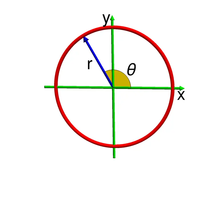
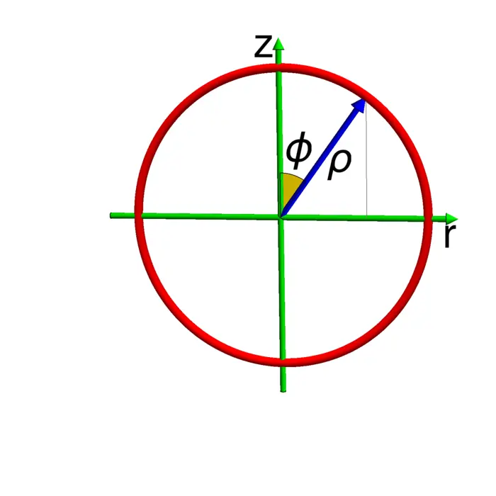
**Figure 3.** Key pictures to derive cylindrical and spherical coordinates.

10.2.7 Spherical Coordinates

The spherical coordinates , where . The angle is the polar angle as in cylindrical coordinates and is the angle between the point and the -axis. We have so that and and therefore where , , and .

10.2.8 Coordinate Changes and Partial Derivatives

A coordinate change in the plane is a map . A point is mapped into . We write for the partial derivative with respect to the variable . For example .

where is a matrix called the Jacobian matrix. The determinant is called the distortion factor at .

10.2.9 The Jacobian Matrix for Polar Coordinates

For polar coordinates, we get

Its distortion factor of the Polar map is . We will use this when integrating in polar coordinates.

10.2.10 The Algebra of Complex Transformations

If with is written as then is a rotation dilation matrix which corresponds to the complex number . The algebra is the same as the algebra of rotation dilation matrices.

10.2.11 Spatial Transformations and the Jacobian

A coordinate change in space is a map . We compute

We wrote . Its determinant is a volume distortion factor.

10.2.12 Volume Distortion in Spherical Coordinates

For spherical coordinates, we have The distortion factor is .

10.3 EXAMPLES

Example 1. The point corresponds to the complex number . It has the polar coordinates . As we have , we check which agrees with

Example 2.

corresponds to spherical coordinates .
The point given in spherical coordinates as is the point .

Example 3.

The set of points with in form a circle.
The set of points with in form a sphere.
The set of points with spherical coordinates are points on the positive -axis.
The set of points with spherical coordinates form a half plane in the -plane.
The set of points with form a sphere. Indeed, by multiplying both sides with , we get which means , which is after a completion of the square equal to .

Example 4. For , has and factor .

Example 5. Find the Jacobian matrix and distortion factor of the map Answer: Write both the transformation and the Jacobian: The Jacobian matrix is .

10.4 ILLUSTRATIONS

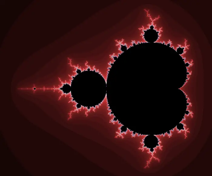
10.4.1 Mandelbrot’s Complexity

Let be defined as , where . The set of all for which the iterates stay bounded is the Mandelbrot set . For we get , so that is either or . The point is in . The point gives , , . Induction shows that does not converge. The point is not in .

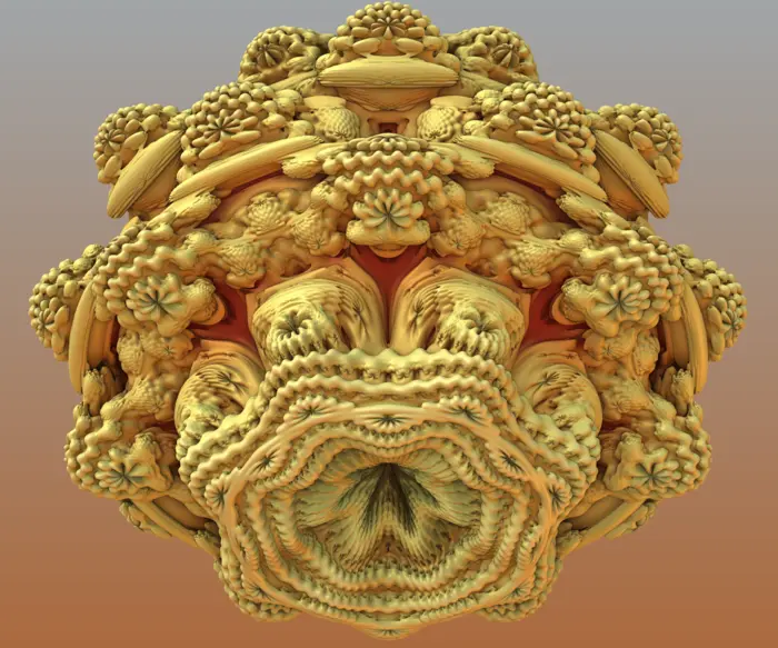
10.4.2 Mandelbrot to Mandelbulb

If is the transformation in which is in spherical coordinates given by , where has spherical coordinates if has . It turns out that gives a nice analogue of the Mandelbrot set, the Mandelbulb.

**Figure 4.** The **Mandelbrot set** . There is a similar construction in space which uses spherical coordinates. This leads to the **Mandelbulb set** , where has spherical coordinates if has spherical coordinates .

EXERCISES

Exercise 1.

Find the polar coordinates of .
Which point has the polar coordinates ?
Find the spherical coordinates of the point .
Which point has the spherical coordinates ?

Exercise 2.

Compute for for , , . Is in the Mandelbrot set?
What is the "eye for an eye" number ? (You can use ).

Exercise 3.

Which surface is described as ?
Describe the hyperbola in polar coordinates.
Which surface is described as ?
Describe the hyperboloid in spherical coordinates.

Exercise 4.

Compute the Jacobian matrix and distortion factor of the coordinate change (Chirikov map).
Compute the Jacobian matrix and distortion factor of the coordinate change (Classical Hénon map).

P.S. When you do the coordinate change of the Chiriov map again and again, one can observe chaos. In the case of the Hénon map, one sees a strange attractor, a fractal object which similarly as the Koch curve encountered last week has a dimension larger than .

Exercise 5.

Verify that the Mandelbrot set is contained in the set . As a reminder, this means you have to show that then escapes to infinity.
Optional: Use the same argument to see that the Mandelbulb set is contained in the set .

Descartes: La Géometrie, 1637 (1 year after the foundation of Harvard college)↩︎
D. Wells, Which is the most beautiful?, Mathematical Intelligencer, 1988.↩︎

Table of Contents